机器学习：多元线性回归闭式解（Python）

import numpy as np
import matplotlib.pyplot as plt


class LRClosedFormSol:
    def __init__(self, fit_intercept=True, normalize=True):
        """
        :param fit_intercept: 是否训练bias
        :param normalize: 是否标准化数据
        """
        self.theta = None  # 训练权重系数
        self.fit_intercept = fit_intercept  # 线性模型的常数项。也即偏置bias，模型中的theta0
        self.normalize = normalize  # 是否标准化数据
        if normalize:
            self.feature_mean, self.feature_std = None, None  # 特征的均值，标准方差
        self.mse = np.infty  # 训练样本的均方误差
        self.r2, self.r2_adj = 0.0, 0.0  # 判定系数和修正判定系数
        self.n_samples, self.n_features = 0, 0  # 样本量和特征数

    def fit(self, x_train, y_train):
        """
        模型训练，根据是否标准化与是否拟合偏置项分类讨论
        :param x_train: 训练样本集
        :param y_train: 训练目标集
        :return:
        """
        if self.normalize:
            self.feature_mean = np.mean(x_train, axis=0)  # 按样本属性计算样本均值
            self.feature_std = np.std(x_train, axis=0) + 1e-8  # 样本方差，为避免零除，添加噪声
            x_train = (x_train - self.feature_mean) / self.feature_std  # 标准化
        if self.fit_intercept:
            x_train = np.c_[x_train, np.ones_like(y_train)]  # 添加一列1，即偏置项样本
        # 训练模型
        self._fit_closed_form_solution(x_train, y_train)  # 求闭式解

    def _fit_closed_form_solution(self, x_train, y_train):
        """
        线性回归的闭式解，单独函数，以便后期扩充维护
        :param x_train: 训练样本集
        :param y_train: 训练目标集
        :return:
        """
        # pinv伪逆，即(A^T * A)^(-1) * A^T
        self.theta = np.linalg.pinv(x_train).dot(y_train)  # 非正则化
        # xtx = np.dot(x_train.T, x_train) + 0.01 * np.eye(x_train.shape[1])  # 按公式书写
        # self.theta = np.dot(np.linalg.inv(xtx), x_train.T).dot(y_train)

    def get_params(self):
        """
        返回线性模型训练的系数
        :return:
        """
        if self.fit_intercept:  # 存在偏置项
            weight, bias = self.theta[:-1], self.theta[-1]
        else:
            weight, bias = self.theta, np.array([0])
        if self.normalize:  # 标准化后的系数
            weight = weight / self.feature_std.reshape(-1)  # 还原模型系数
            bias = bias - weight.T.dot(self.feature_mean.reshape(-1))
        return np.r_[weight.reshape(-1), bias.reshape(-1)]

    def predict(self, x_test):
        """
        测试数据预测，x_test：待预测样本集，不包括偏置项1
        :param x_test:
        :return:
        """
        try:
            self.n_samples, self.n_features = x_test.shape[0], x_test.shape[1]
        except IndexError:
            self.n_samples, self.n_features = x_test.shape[0], 1  # 测试样本数和特征数
        if self.normalize:
            x_test = (x_test - self.feature_mean) / self.feature_std  # 测试数据标准化
        if self.fit_intercept:
            x_test = np.c_[x_test, np.ones(shape=x_test.shape[0])]  # 存在偏置项，添加一列1
        return x_test.dot(self.theta)

    def cal_mse_r2(self, y_pred, y_test):
        """
        计算均方误差，计算拟合优度的判定系数R方和修正判定系数
        :param y_pred: 模型预测目标真值
        :param y_test: 测试目标真值
        :return:
        """
        self.mse = ((y_test - y_pred) ** 2).mean()  # 均方误差
        # 计算测试样本的判定系数和修正判定系数
        self.r2 = 1 - ((y_test - y_pred) ** 2).sum() / ((y_test - y_test.mean()) ** 2).sum()
        self.r2_adj = 1 - (1 - self.r2) * (self.n_samples - 1) / (self.n_samples - self.n_features - 1)
        return self.mse, self.r2, self.r2_adj

    def plt_predict(self, y_pred, y_test, is_show=True, is_sort=True):
        """
        绘制预测值与真实值对比图
        :return:
        """
        if self.mse is np.infty:
            self.cal_mse_r2(y_pred, y_test)
        if is_show:
            plt.figure(figsize=(7, 5))
        if is_sort:
            idx = np.argsort(y_test)
            plt.plot(y_pred[idx], "r:", lw=1.5, label="Predictive Val")
            plt.plot(y_test[idx], "k--", lw=1.5, label="Test True Val")
        else:
            plt.plot(y_pred, "r:", lw=1.5, label="Predictive Val")
            plt.plot(y_test, "k--", lw=1.5, label="Test True Val")
        plt.xlabel("Test sample observation serial number", fontdict={"fontsize": 12})
        plt.ylabel("Predicted sample value", fontdict={"fontsize": 12})
        plt.title("The predictive values of test samples n MSE = %.5e, R2 = %.5f, R2_adj = %.5f"
                  % (self.mse, self.r2, self.r2_adj), fontdict={"fontsize": 14})
        plt.legend(frameon=False)
        plt.grid(ls=":")
        if is_show:
            plt.show()


from sklearn.datasets import fetch_california_housing
from sklearn.model_selection import train_test_split
from sklearn.linear_model import LinearRegression
from sklearn.metrics import r2_score, mean_squared_error


housing = fetch_california_housing()
X, y = housing.data, housing.target  # 获取样本数据和目标数据
X_train, X_test, y_train, y_test = 
    train_test_split(X, y, test_size=0.3, random_state=1, shuffle=True)

lgcfs_obj = LRClosedFormSol(normalize=True, fit_intercept=True)
lgcfs_obj.fit(X_train, y_train)
theta = lgcfs_obj.get_params()  # 获得模型系数
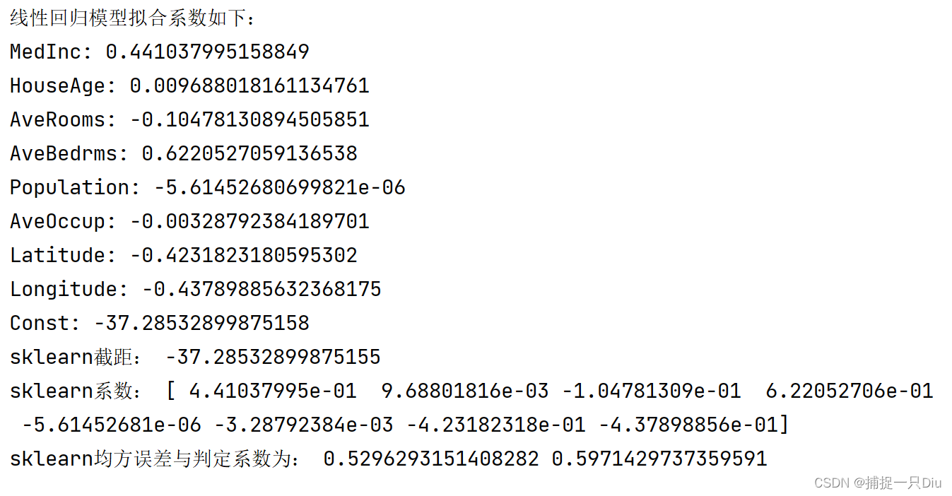
print("线性回归模型拟合系数如下：")
for i, fn in enumerate(housing.feature_names):
    print(fn + ":", theta[i])
print("Const:", theta[-1])

# 模型预测，即针对测试样本进行预测
y_pred = lgcfs_obj.predict(X_test)
lgcfs_obj.plt_predict(y_pred, y_test, is_sort=True)

# 采用sklearn库函数进行线性回归和预测
lr = LinearRegression().fit(X_train, y_train)
print("sklearn截距：", lr.intercept_)  # 打印截距
print("sklearn系数：", lr.coef_)  # 打印模型系数
y_test_predict = lr.predict(X_test)
mse = mean_squared_error(y_test, y_test_predict)
r2 = r2_score(y_test, y_test_predict)
print("sklearn均方误差与判定系数为：", mse, r2)

代码007普通

打赏 收藏 海报 链接